 |
|
|
|
|
|
|
|
|
|
Research  |
|
|||||||||||||||||||||||||||||||||||||||||||||||||
| research home | special topics home | ||||||||||||||||||||||||||||||||||||||||||||||||||
| Special Topics | ||||||||||||||||||||||||||||||||||||||||||||||||||
|
|
||||||||||||||||||||||||||||||||||||||||||||||||||
|
Signal Processing Techniques by John A. Putman M.A., M.S. |
||||||||||||||||||||||||||||||||||||||||||||||||||
The Fourier Transform
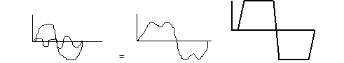
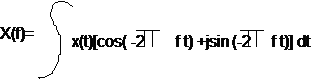
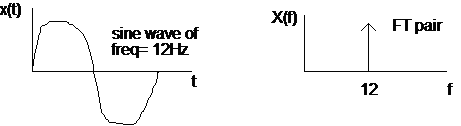
For example: fig.a shows a fundamental frequency with its 3rd harmonic. Combining them, we get a composite wave form that looks something like fig.b. If we combine enough harmonics of increasing frequency and decreasing amplitude, we end up with a near perfect "square" wave (fig.c). There are two types of Fourier Analysis. The first is Fourier Series analysis for periodic signals (i.e. signals that have exactly the same pattern for each cycle, such as quasars, 60Hz wall current noise or regular heart beats -also referred to as time invariant signals). The second form of analysis is called the Fourier transform which deals with non periodic signals such as the human EEG which varies continuously over time. Thus the Fourier transform of a non- periodic signal produces a continuous transform. When the input signal is periodic (repeats itself exactly with each cycle) its frequency content can be represented by a discrete set of numbers called the Fourier series coefficients. They signify the "weight" given each frequency that is required to reconstruct the original signal. Furthermore, the frequencies that correspond to these different coefficients are harmonically related ; each being an integer multiple of some fundamental frequency. This paper will confine itself primarily to exploring the background and application of the Fourier transform since this is the signal processing technique utilized in Neurofeedback (the EEG being intensely non-periodic). The Fourier transform is one of the most commonly used methods of signal analysis. It is simply a mathematical transformation that changes a signal from a time domain representation to a frequency domain representation thereby allowing one to observe and analyze its frequency content. Plotting a Fourier transform gives us a visual representation of the relative proportion of different frequencies in an input signal. Some examples: the FT of single sine wave would appear as a single spike (see below), indicating that only one frequency was present. Similarly, the noise from florescent lights appears as a prominent peak at 60 Hz. Where as the processing of a periodic signal with the Fourier series produces a discrete set of coefficients, a non-periodic signal requires a mathematical tool that will produce a continuous transform (i.e. one that changes continuously over time instead of the photo-like transform of the periodic signal) . The Fourier transform therefore, requires something a bit more powerful. When moving from the time domain x(t) into the frequency domain X(f), the time function x(t) must be evaluated for all values of t (time). The following is the actual Fourier transform which illustrates the mathematical relationship between the time domain x(t) and the frequency domain X(f).
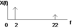
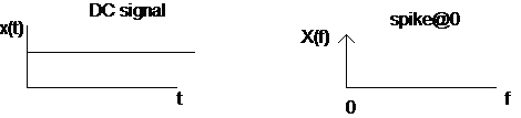
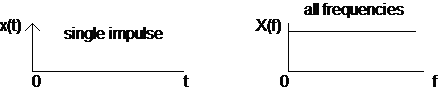
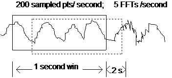
The product of the time function x(t) and a [complex trigonometric expression] yield the frequency function X(f) when integrated over time t for a specific frequency f (Integration involves finding the area defined by a specific function over small increments, in this case dt.) Go over that last sentence slowly three more times and then please note: Although mathematical formulas will appear in this paper they are more for historical significance than anything else. The emphasis will be on developing an intuitive understanding of the concepts discussed. Here are some examples of signals in the time domain and their corresponding Fourier transform: 1.) 2.) transforms to: 3.) 4.) Regarding examples 3 and 4: Signals that are narrow in the time domain (e.g. an impulse) are wide in the frequency domain (flat line of same amplitude). Conversely, signals that are wide in the time domain (e.g. DC signal flat line) are narrow in the frequency domain (impulse w/ frequency =0). Also note: For our purposes in the field of EEG biofeedback, the magnitude of each frequency is often all that is shown on a spectral display. However for the complete reconstruction of a signal, phase information is necessary as well. The following is an example of a fast Fourier transform performed on a wave form similar to those used in EEG biofeedback. Note that a "fast" Fourier transform (or FFT) is simply a computationally efficient algorithm designed to speedily transform the signal for real time observation.
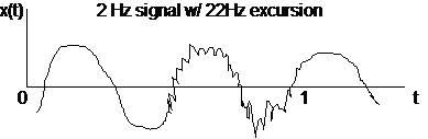
The dominant frequency of this signal is approximately 3.5 Hz. The instrument samples the input signal at a rate of 200 times per second and performs FFTs at a rate of 5 per second (a little on the slow side as FFTs go.) Notice that the sampling rate is not the same thing as the FFT rate! The sampling rate is the frequency with which the data points are gathered while the FFT rate is an indication of how often the mathematical operation is performed on the sampled points. Sampling rate does, however, play a role in the ultimate resolution of the displayed signal. The width of the FFT window in this case is 1 second (a window is a defined period of time within which a mathematical operation is performed). Since the FFT rate is 5 /second, a new FFT is calculated every .2 seconds. Having a window of 1 second implies that .8 seconds of old data is being averaged in with the .2 seconds of new data. This process is known as "smoothing" in that the response is a bit more sluggish to the eye of the patient. The smaller the ratio of new data to old, the slower the response of the feedback. Conversely, if we were to narrow the FFT window to .2 seconds (matching the FFT rate in this case and eliminating old data from the average), we would have zero smoothing leading to a highly reactive and what many would consider, agitating form of feedback. In this case an FFT window of less than .2 seconds would, of course, leave gaps in the sampled data. Filters
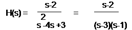
So how does a filter actually remove unwanted frequencies? This is accomplished by sending the input signal through a system function H(s) which determines the degree of amplification for each frequency in the signal. The desired frequencies are boosted by the instrument gain while the unwanted frequencies are boosted by a gain of zero. The following is the general form of a system function: H(s) = g(s) / x(s) where "s" represents a complex frequency. (Note that the term "complex" refers to a combination of real and imaginary numbers - specifically the square root of (-1) which, technically, does not exist. Hence the name "imaginary" number. The concept of complex numbers is just a mathematical trick to keep our equations happy and running smoothly and will not be discussed further.) The frequencies to be eliminated are those for which H(s) = 0. More specifically, they are the roots of the function g(s) (i.e. those values of s which make g(s) = 0). The solutions are referred to as zeros. Conversely, the roots of the function in the denominator, x(s), are those that cause H(s) to go to infinity (maximum gain). Solutions to x(s) are referred to as "poles." For example:
This implies that s =2 is a zero; and s =1 and s = 3 are poles. VOILA'!! We have just created a simple filter.
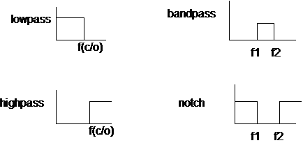
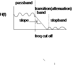
Designing a filter involves nothing more than designing a system function that has the desired frequency response (i.e. placing the poles and zeros in the correct configuration in the frequency plane to obtain the desired waveform). This response is known as a "Bode plot" named after (who else?) Dr Bode. A computer is generally used to determine the roots (pole/zero locations) of the appropriately chosen polynomials. These can be found in most filter design or operational amplifier textbooks. Obviously there is no such thing as an "ideal" filter. The frequency response of most filters look something like the following low pass filter. Terms: Transition band: the band over which the frequency response transitions from the pass band to the stop band. Attenuation: this refers to the degree of difference between the pass band and stop band. Attenuation rate: refers to the slope or roll off rate. Usually measured in dBs (decibels) per octave. Note that an octave is a doubling of a frequency (e.g. the difference in pitch between C1 and C2 on a piano). Cutoff frequency: the edge of the pass band; also called the corner frequency. Gain: the amount of amplification of the signal in the pass band. Order: the number of poles in the system function H(s) (equal to the highest degree of the polynomial in the denominator). The higher the order, the steeper the roll-off (see below). Higher order filters are more complicated to build.
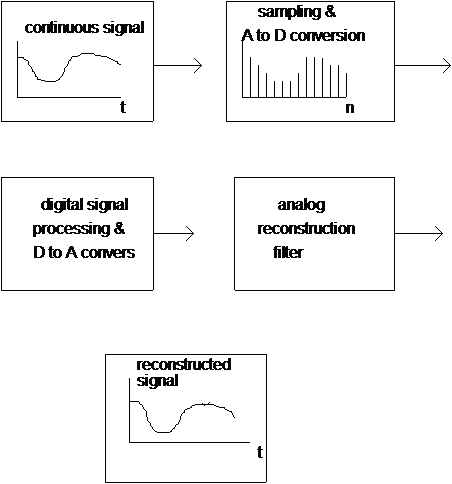
Phase Response Sampling
So why all the bother? Why not simply leave everything in the analog domain and be happy? The reason is that signal processing in the digital domain, with all of its complexity, gives us much greater flexibility. For instance; changing filter characteristics involves reprogramming a few numbers rather than pulling out and replacing resistors and capacitors. Aliasing
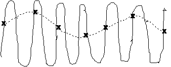
Example: a high frequency signal that is sampled too slowly. The laws of signal processing dictate that the lowest frequency sine wave (the dotted trace) that will fit the sampled data points will be the frequency that gets integrated into the reconstructed analog signal. In the above example, the sampled points are simply too sparse for an accurate reconstruction of the high frequency signal (solid trace). In this case, aliasing will tend to corrupt the low end of the frequency spectrum making it appear that there is more low frequency activity than may actually occurring. The frequency at which a signal aliases f(a) is equal to the difference between the sampling frequency f(s) and the maximum frequency f(m) in the band being measured. or f(a) = f(s) - f(m) In all cases, the value of f(s) must always be at least twice that of f(m). But just for fun , let's assume otherwise. Let's say: f(s) < 2f(m) If this is so then f(s) - f(m) < f(m) which implies that f(a) < f(m). What this means is that the frequency at which we experience aliasing is less than the maximum frequency of the signal in the band. Bad news! Here is an example involving actual numbers: Let's say f(s) = 30Hz and f(m) = 18Hz. Then f(a) = 30 Hz - 18Hz = 12Hz. This means that we will begin to experience signal corruption beginning at 12 Hz, well within the band we are interested in measuring. Thus, it is vital that the sampling rate always be greater than twice the maximum frequency being measured: f(s) > 2f(m). This rule is known as The Nyquist Sampling Theorem. To ensure that aliasing does not occur in the sampling process, the signal to be sampled is passed through a lowpass filter to impose the appropriate band limitations on the signal. This filter is known as an anti-aliasing filter. Another method of ensuring the integrity of signal reconstruction is called over-sampling. The Nyquist theorem states that it is possible to completely reconstruct a signal as long as the sampling rate is at least twice the maximum frequency in the signal. The closer to the Nyquist threshold the signal, the sharper (higher order) the analog low pass filter required to band limit the signal (i.e. the roll off must be very steep). Rather than constructing one of these monster filters, the technique of over-sampling is used. In this way the sampled points are close enough together so a more realistic low-pass filter can be used. As an example: CD players are advertised as having 4x or 8x over-sampling. The human auditory system cannot hear frequencies higher than 20KHz. The typical CD contains audio information sampled at a rate of 44KHz. Typical sampling rates for EEG biofeedback is 150 samples per second or greater. This means that the EEG biofeedback process generally involves frequencies that are below 75 Hz. Amplifiers and Voltage Laws Charge: The quantity of electricity. Unit symbol: C for Coulomb which is 6.242 x 10 to the 18th power number of electrons (or protons). Current: Represented by the symbol " i ". Unit measure is the ampere (A). A flow of charge equivalent to 1 Coulomb per second. Voltage: Symbol: V or E. Unit is the Volt (V). The amount of electromotive force pushing current between two points. Resistance: Symbol: R. Unit is the ohm. The ratio of voltage divided by current for a given conductor under a given set of conditions. A form of Impedance (see below) related to DC circuits ( i.e. circuits with currents that flow in one direction at a relatively constant rate). Reactance: Symbol: (usually X). Unit is the ohm. The part of impedance of an AC circuit ( i.e. a circuit with currents that reverse (alternate) direction due to capacitance and/ or inductance). Impedance: Symbol: Z. Unit is the ohm. The vector combination of resistance and reactance. Impedance is an apparent force that is in opposition to the flow of current in a circuit. Ohms Law Kirchhoff's Voltage Law
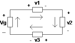
Kirchhoff's law is a result of the fact that the output of a voltage generator (Vg) is equal to the sum of the voltage drops across the resistive elements within the circuit: which implies that: Note that -(Vg) is actually a negative voltage drop since it is the output of the generator (in other words it represents a voltage rise). This law will prove very important regarding the subject of electrode vs. amplifier input impedance which we will now consider. Impedance When current flows through a closed loop, it is analogous to water flowing through a hose. In other words the amount of water (current) that enters the hose (loop) is the same amount that comes out the other end. And like a hose, if there is a difference in the amount of current flowing past any two different points in the circuit, then there is a current drain somewhere in the circuit. (This is the principle on which the ground fault interrupter works in biofeedback instrumentation to insure against an electrical shock to the patient. When the GFI detects a current drop between the live wire and a neutral location in the circuit, a breaker is triggered that shuts down the system.) In the following example we will examine how this feature of current and Kirchhoff's Voltage Law explain one of the reasons behind the importance of low electrode impedance and high input instrument impedance when performing EEG biofeedback. For simplicity and for reasons that will become clear later in this paper, we will only be dealing with the resistance component of impedance.
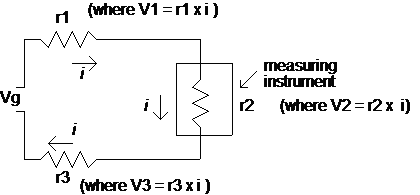
Remember that the current ( i ) that flows through each element (r1, r2 and r3) is exactly the same. (Note that r2 is the input impedance of the measuring instrument). In order to have maximum accuracy in measuring the voltage being generated (Vg), the voltage drop across the measuring instrument (V2) must be very close to Vg. Thus we want the voltage drop (V1 andV3) across r1 and r3 to be minimal. (r1 and r3 can represent the contact resistance of the biofeedback sensors). Since, according to Kirchhoff's Law, Vg = V1 + V2 + V3 , we want V1 and V3 to be negligible in order for V2 to be as close to Vg as possible. Since the current is the same across each element, the only way we can obtain this outcome is by controlling the impedance (i.e. very LOW contact resistance at r1 and r3 with very HIGH instrument input impedance at r2) . This is why it is common to see instruments with whopping impedances of 1 million meg-ohms (that's a million -million ohms folks !). When compared to the voltage drop at the contact sensors (due to 5000 to 10,000 ohm contact resistance) we can see that the voltage loss is fairly insignificant. However there is a much more crucial issue concerning the importance of low contact resistances, as we shall soon see. Differential Amplifiers
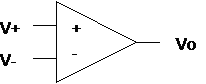
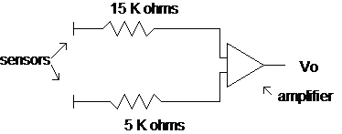
Vo = A [( V+) - (V-)] A differential amplifier with a very high gain and extremely high input impedance is called an operational amplifier or simply an "op-amp." The inputs have extremely high impedances and the output node has near zero resistance allowing it to behave like an ideal voltage source supplying as much current as is necessary. In order to get a sense of how a differential amplifier works, think of 2 microphones at the extreme ends of a choir with sopranos placed at one end and bassos at the other. In the middle (approximately equidistant from the 2 mics) place the midrange voices -altos, contraltos, tenors, etc. If this were a non -differential amplifier (several mics on separate channels placed around the choir) all of the voices would be amplified to the same degree. However a differential amplifier would only amplify the sopranos and bassos. Why? Because the sound from the midrange voices would arrive at both microphones simultaneously with the same intensity and frequency causing the input at both mics to be exactly the same thus cancelling each other out. This quality, unique to differential amplifiers, is referred to as common mode rejection. The signals that are common to both inputs cancel themselves out while the signals that are unique to each input are preserved for amplification. In the field of EEG biofeedback this particular feature of the differential amplifier becomes critically important. The reason for this is that we tend to work in an extremely polluted environment from an electromagnetic standpoint. Anytime electric current is run through a circuit, an electromagnetic field forms around the device and extends out into space anywhere from a few feet to a few miles. As such, the feature of common mode rejection becomes one of the technicians greatest ally in attaining clean measurements. So what are some of the sources of common mode input? Basically, it is any power source that is far enough away to influence each electrode to nearly the same degree. These can include: computers, power outlets, radios, motors, ignition switches, generators, florescent lights and toaster ovens. Electric Fields In addition, it is almost inevitable that an imbalance will exist between the electrode skin resistance of the two electrodes which, if large enough, can completely defeat the common mode rejection feature of the differential input system. A significant difference in the electrode impedances can change a common mode signal (which is subject to complete cancellation) to a differential mode signal resulting in corruption of the measurement. This is why low electrode impedances (contact resistance) are important for accurate readings. For example: Let's say that an electro-magnetic field induces a current flow of 0.2 nA (nano amperes) on the above system. A nano amp is equal to 0.000,000,001 amps. The above simplified schematic represents two electrodes with skin resistances of 15 K ohms and 5 K ohms leading into the differential amplifier. Using Ohms Law would give us a voltage of : 0.2 nA x 15 K ohms = 3.0 uV at the top electrode -skin interface. and 0.2 nA x 5 K ohms = 1.0 uV at the bottom electrode skin interface. This would lead to a differential voltage of: 3.0 uV - 1.0 uV = 2.0 uV. Thus Vo would include this added 2.0 uV in its output to the computer for analog reconstruction. Since we are concerned with the difference between the electrode-skin resistances, we could actually have resistances as high as we wanted so long as the difference between them remained small (correspondence from Siegfried Othmer). However it is difficult to have high electrode -skin resistances that would be close enough to each other in value to sufficiently cancel the extraneous voltage. Keeping both of them under 5,000 ohms will give us a reasonable margin given the extremely small common mode currents we deal with in performing EEG biofeedback. Impedance vs. Resistance Revisited Reference John Daintith and R.D. Nelson. Dictionary of Mathematics. Penguin Books, New York, NY 1989. Eric Donker, Shakib Saria, Electronic Devices and Circuits. NTC Contemporary Publishing, Chicago, Ill 1998. Zoher Z. Karu Signals and Systems Made Ridiculously Simple. ZiZi Press, Huntsville, AL 1995. Alan V. Oppenheim, A.S. Willsky, and I. Young. Signals and Systems. Englewood Cliffs, NJ: Prentice -Hall, 1983. Daniel L. Metzger. Electronics Pocket Handbook. Second Edition. Englewood Cliffs, NJ: Prentice -Hall, 1992. I. S. Sokolnikoff and R.M. Redheffer. Mathematics of Physics and Modern Engineering. McGraw-Hill Book Company, New York, NY 1966. Toomim Hershel. Bioelectric Concepts. Unpublished manuscript. 1989. |
||||||||||||||||||||||||||||||||||||||||||||||||||